Symmetrical and Asymmetrical Data
It has been observed that the natural variation of many variables tends to follow a bell-shaped distribution, with most values clustered symmetrically near the mean and few values falling out on the tails. This referred to as the normal distribution.
With a normally distributed bell curve, the mean, median and mode all fall on the same value.
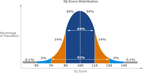
Below is an example of the bell curve of normal distribution for IQ
The way one reads the normal distribution is as follows:
Firstly, ignore the numbers within the chart at this point, we will refer to them later on in the module.
Along the x-axis is what you are measuring, in this example IQ. Along the y-axis is the percentage of the population that corresponds to the value along the x-axis. With a normal distribution of data, the values in the middle of the curve on the x-axis occur frequently, and as one moves away from the middle (to either side) the percentage of the population that have the corresponding IQ drops.
In this example, the average (or mean) IQ value is 100. An IQ of 100 is also the mode as it occurs most frequently and is also the median as it is in the middle of the data set. As one moves away from the IQ of 100, either above or below 100, the frequency of its occurrence diminishes. This is a normally distributed data set.
As mentioned earlier, the mean value of a data set can be used to predict future occurrences when the data is symmetrical, and this can be explained by the graph above. If you were to guess what the IQ of a random person on the street was, one could be fairly confident it would fall close to the average IQ of 100, as 68% of all individuals IQs fall between 85 and 115.